Key takeaways
What you will learn
- The right model is the one whose mathematical assumption matches your lens’s physical projection.
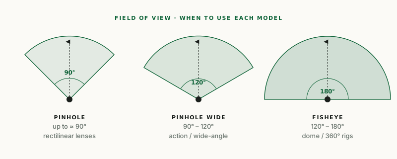
- Pinhole works up to about 90° FOV; pinhole-wide stretches to ~120°; fisheye covers the rest up to 180°.
- A wrong model produces a high RMS even on clean captures — fitting a fisheye lens with a pinhole model is the most common mismatch.
- When in doubt, solve the same images against several models in CalibrX and compare RMS plus undistortion previews directly.
Why "model" is the first calibration decision
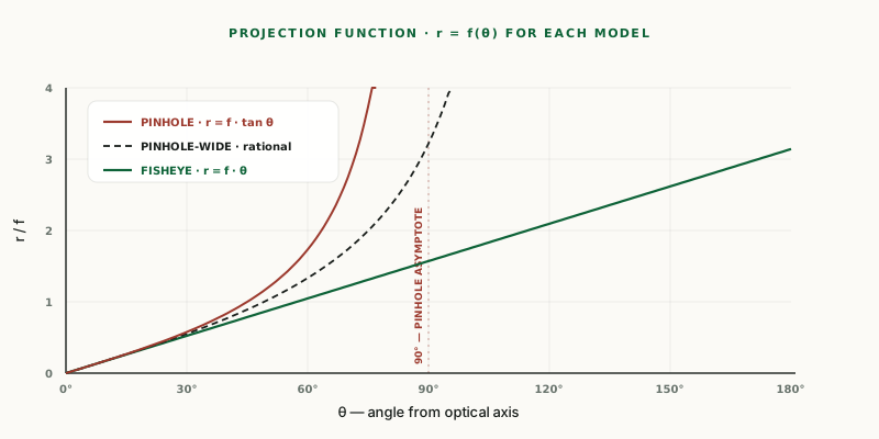
Every camera-calibration solver makes a mathematical assumption about how light from a 3D world point lands on a pixel. The pinhole assumption says light travels in a straight line through a single point; the fisheye assumption says angle from the optical axis maps linearly to image radius; the rational pinhole splits the difference. The optimisation then finds the parameters within that family that fit the observed data best.
When the assumption matches your lens, the fit converges to a small reprojection error and the undistorted images look natural. When it does not, you are forcing the solver to explain a fisheye captures with a pinhole formula — like trying to fit a circle with a straight line. The optimiser will still return something, but the result is unusable: high RMS, severe warping at the edges of the undistorted image, and downstream pipelines that misbehave.
CalibrX supports three model families precisely because no single one covers every lens. Picking between them is the first real calibration decision, made before you even capture an image.
The standard pinhole (Brown–Conrady)
The basic pinhole projection is , where is the angle from the optical axis and is the radial distance in the image plane. This is the textbook model and it works extremely well for ordinary lenses — phone cameras, machine-vision lenses, most webcams. Distortion is added on top with the polynomial
The model breaks down geometrically as approaches , where diverges to infinity. In practice this means: a 70° FOV lens is comfortable, an 85° FOV lens is borderline, and anything past 100° starts producing high RMS and bad edge behaviour because the polynomial cannot bend the projection sharply enough to keep up with reality.
For typical industrial vision, security cameras, drone front cameras, and consumer phones, the standard pinhole is the right default. The distortion vector has enough flexibility to capture most lens behaviour without being so flexible that it overfits noisy captures.
The rational pinhole (pinhole-wide)
The rational model uses the same pinhole projection but extends the distortion polynomial with a denominator:
This rational form gives the optimisation more degrees of freedom to bend the projection curve at larger angles. It pushes the usable range of the pinhole family out to roughly 120° before the underlying assumption breaks. CalibrX calls this model `pinhole_wide`; OpenCV exposes it as the `CALIB_RATIONAL_MODEL` flag on `calibrateCamera`.
Use pinhole-wide for action cameras with the standard (non-fisheye) lens setting, automotive forward cameras with wide FOV, drone cameras with rectilinear wide-angle lenses, and AR/VR pass-through cameras. The extra coefficients cost a little robustness — you need a few more frames with good edge coverage to constrain them — but the payoff is a much better fit at the corners of the image.
The fisheye model (Kannala–Brandt)
True fisheye lenses violate the pinhole assumption fundamentally: they do not project light through a single mathematical point. Their projection law is approximately equidistant, , meaning angle from the optical axis maps linearly to image radius. That linear relationship is bounded — it stays finite at — which is what lets a 180° lens map an entire hemisphere onto a flat sensor.
The Kannala–Brandt model parameterises the projection with a polynomial in : This is what OpenCV implements in the `cv2.fisheye` namespace and what CalibrX uses for the `fisheye` model. Note the polynomial is in (the angle) rather than in (the radius) — that is the mathematical reason fisheye is a different model rather than a more aggressive pinhole.
Use the fisheye model for true fisheye lenses (any lens marketed as fisheye or 180°), GoPro footage shot in wide or superview modes, dome cameras, multi-camera 360° rigs, and circular fisheye captures where the image actually shows a black circle in the corners of a rectangular frame.
How to choose — a practical flow
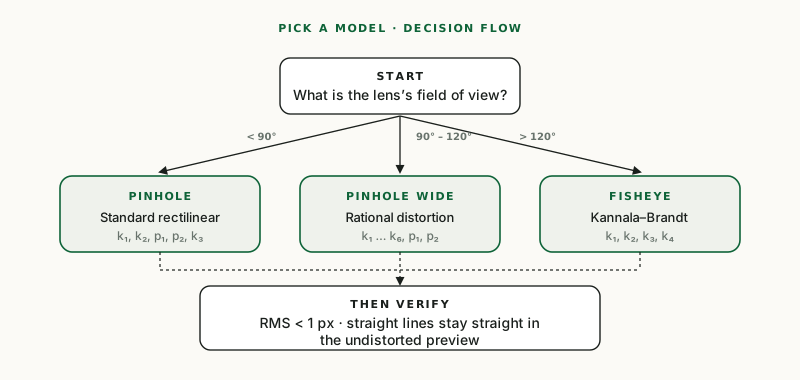
In practice you have two cheap signals to guide the choice. The first is the lens’s nominal field of view: most lenses are sold with a FOV spec, and that spec immediately suggests a model family. The second is the appearance of straight world lines in the raw image: if a printed straight edge curves dramatically toward the corners, you are almost certainly in fisheye territory.
When you can afford it, the most robust approach is to solve the same captures against multiple models and compare them side by side. CalibrX shows the RMS reprojection error for each solved model and lets you preview the undistortion. The right model usually wins on both axes simultaneously — lowest RMS and cleanest straight lines in the undistorted preview. If two models tie on RMS, prefer the one with fewer parameters (pinhole over pinhole-wide; pinhole-wide over fisheye) to avoid overfitting.
- Lens FOV is under 90°: start with standard pinhole.
- Lens FOV is 90° – 120°: try pinhole-wide first.
- Lens FOV is above 120° or the lens is marketed as fisheye: use the fisheye model.
- Verify by checking RMS and inspecting the undistorted output — straight world lines should stay straight.
- When tied, the simpler model wins.
Common pitfalls
The most common mistake is fitting a fisheye lens with the standard pinhole model. The optimiser converges, returns a high RMS (often above 3 px), and the undistorted output bends straight lines in odd ways near the corners. The signature: edge points get pushed off-screen or smeared into a halo. The fix is to re-solve with the fisheye model — usually drops RMS by a factor of 5–10×.
A subtler mistake is fitting a moderately wide lens with the full fisheye model. The fisheye estimator is hungry for edge coverage and can produce unstable when the captures only reach moderate angles. The result looks numerically fine but the undistortion at the periphery has a "swimming" feel. If pinhole-wide gives comparable RMS, prefer it.
And finally: distortion coefficients beyond the leading two () get unstable when captures lack edge coverage. The polynomial is most constrained at the corners of the sensor, so a calibration set with all the board placements clustered near the centre will leave and the rational denominator coefficients essentially unconstrained — and they can take physically nonsensical values without you noticing in the RMS.
Further reading
- OpenCV — Camera calibration (calib3d) moduleAPI reference for calibrateCamera, the rational distortion model, and the standard Brown–Conrady parameters.
- OpenCV — cv2.fisheye namespaceAPI reference for the equidistant fisheye model used by CalibrX’s fisheye solver.
- Kannala & Brandt — A Generic Camera Model and Calibration Method (2006)The paper behind OpenCV’s fisheye model and the equidistant projection used for wide-angle and 180° lenses.
- Brown — Decentering Distortion of Lenses (1966)The original derivation of the radial + tangential distortion model still used today (Brown–Conrady).
- CalibrX — calibration pattern generatorGenerate printable chessboard, ChArUco, and ArUco targets to capture data for any of these camera models.
- CalibrX — camera calibration without OpenCV or MATLABFit all three models against the same captures in the browser — no OpenCV or MATLAB code required.