Key takeaways
What you will learn
- Camera calibration estimates the parameters that map a 3D world point to its 2D image pixel.
- The intrinsic matrix K describes focal lengths and principal point; the distortion vector D describes how lenses deviate from an ideal pinhole.
- Calibration is a nonlinear least-squares problem: given known 3D–2D correspondences, find K and D that minimise reprojection error.
- RMS reprojection error is the standard quality metric, but per-frame and per-region diagnostics matter more than a single number.
- OpenCV’s calibrateCamera is built on Zhengyou Zhang’s 2000 paper, which made the problem tractable for any flat target.
The mapping from world to pixel
A camera does not record pixels — it records light. Every pixel value in an image is the result of light reflecting off some 3D surface in the world, passing through a lens, and being measured by a sensor element. Camera calibration is the inverse problem: given the pixels, can we describe the geometric function that produced them?
The key to understanding that function is realizing it is not one transformation but a chain of four, passing through four different coordinate systems — each with its own origin. A point travels from the world frame, into the camera frame, onto the image plane, and finally into pixel coordinates. Throughout this article we use a strict convention: capital letters denote the axes of a coordinate system (, , ), while lowercase letters denote the coordinates of a specific point measured along those axes (, , ).
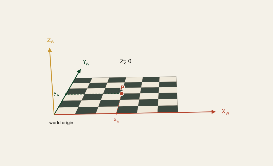
Step 1: the world frame. The world coordinate system is arbitrary — we choose it. In calibration it is typically anchored to the target: the origin sits at a corner of the checkerboard, with and spanning the board plane and perpendicular to it. A point in the scene has world coordinates ; for a point on the board itself, . Nothing about the camera has entered the picture yet — this frame describes the scene, not the sensor.
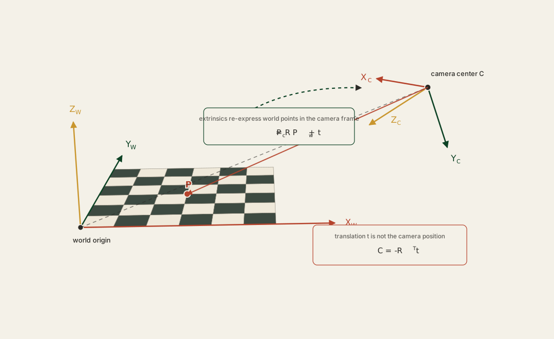
Step 2: the extrinsic transform. The camera has its own coordinate system: its origin is the optical center (the point all rays pass through), with pointing right, pointing down, and pointing forward along the optical axis into the scene. The extrinsic parameters — a rotation and a translation — re-express the point in this frame: It is worth pausing on what this does and does not do. The point has not moved. Only the reference frame has changed: the same physical point now carries new coordinates — its position as seen from the camera. In particular, is the point's depth along the camera's viewing direction, a quantity that simply does not exist in the world frame.
Two properties of the extrinsics deserve precision, because they are the source of endless bugs. First, is not nine free numbers: it is an orthonormal rotation matrix (, ) with only three degrees of freedom, which is why libraries store it compactly as an axis–angle vector (OpenCV's rvec, expanded via the Rodrigues formula). Second — and this is the classic trap — is not the camera's position in the world. Setting in the equation above shows that is the world origin expressed in the camera frame. The camera's actual position in world coordinates is . Report tvec as "camera position" and every downstream measurement will be silently wrong.
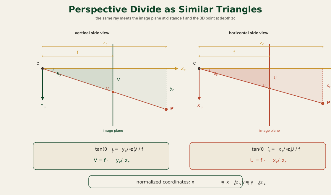
Step 3: the perspective divide. This is the step where a photograph actually happens. An ideal pinhole projects the point onto a plane at unit distance in front of by dividing out the depth: These normalized image coordinates are dimensionless and independent of any particular sensor. The divide is the only nonlinear operation in the entire chain, and it is where information is destroyed: 3D collapses to 2D, depth is gone, and "farther away" becomes "smaller" as a direct consequence of the arithmetic. It is also why a single pixel can never be inverted back to a 3D point — only to a ray of candidate points through , all of which share the same .
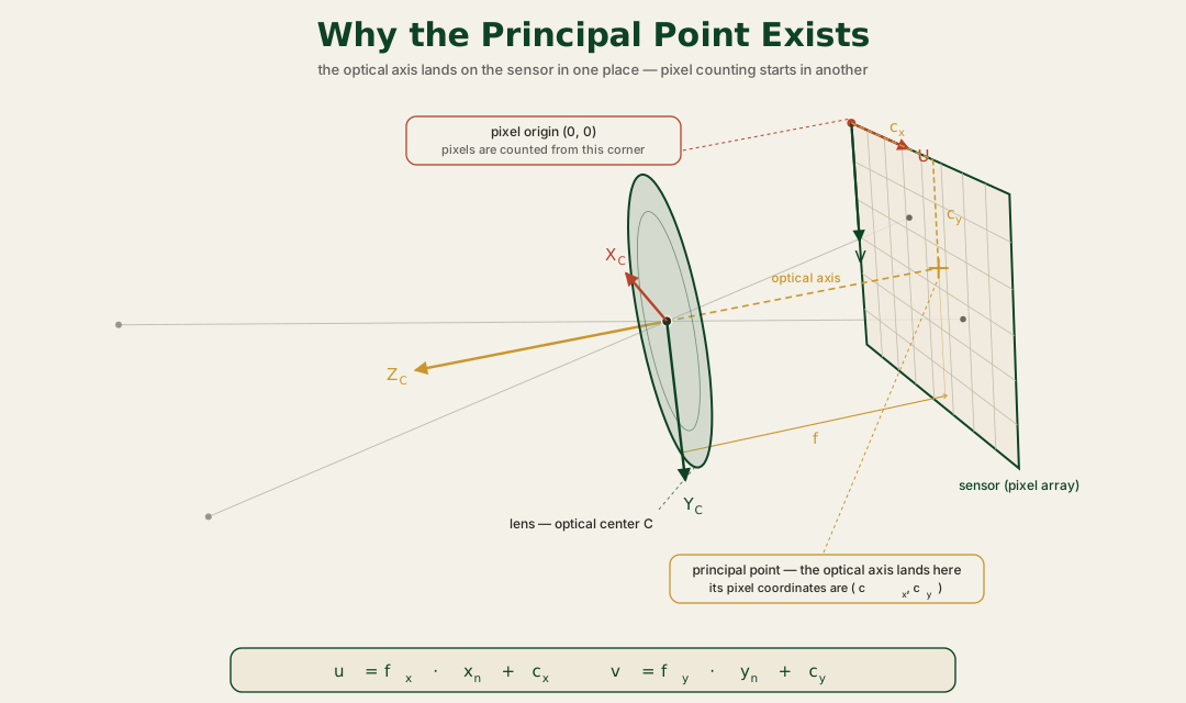
Step 4: the intrinsic matrix. So far no property of the physical camera has appeared — the normalized coordinates would be identical for any ideal pinhole. The intrinsics convert this idealized description into the actual pixel grid of a specific sensor: Here and are the focal lengths expressed in pixels — the lens focal length multiplied by the sensor's pixel density — which is why a "35 mm" lens produces values in the thousands. They control how many pixels one unit of normalized coordinate spans: the magnification. The principal point handles a bookkeeping fact: the projection is naturally centered on the optical axis, but images are indexed from the top-left corner. The offset is the pixel location where the optical axis pierces the sensor — near the image center, but never exactly, which is why it is estimated rather than assumed. Packed as a matrix, with a skew term that is effectively zero on modern sensors:
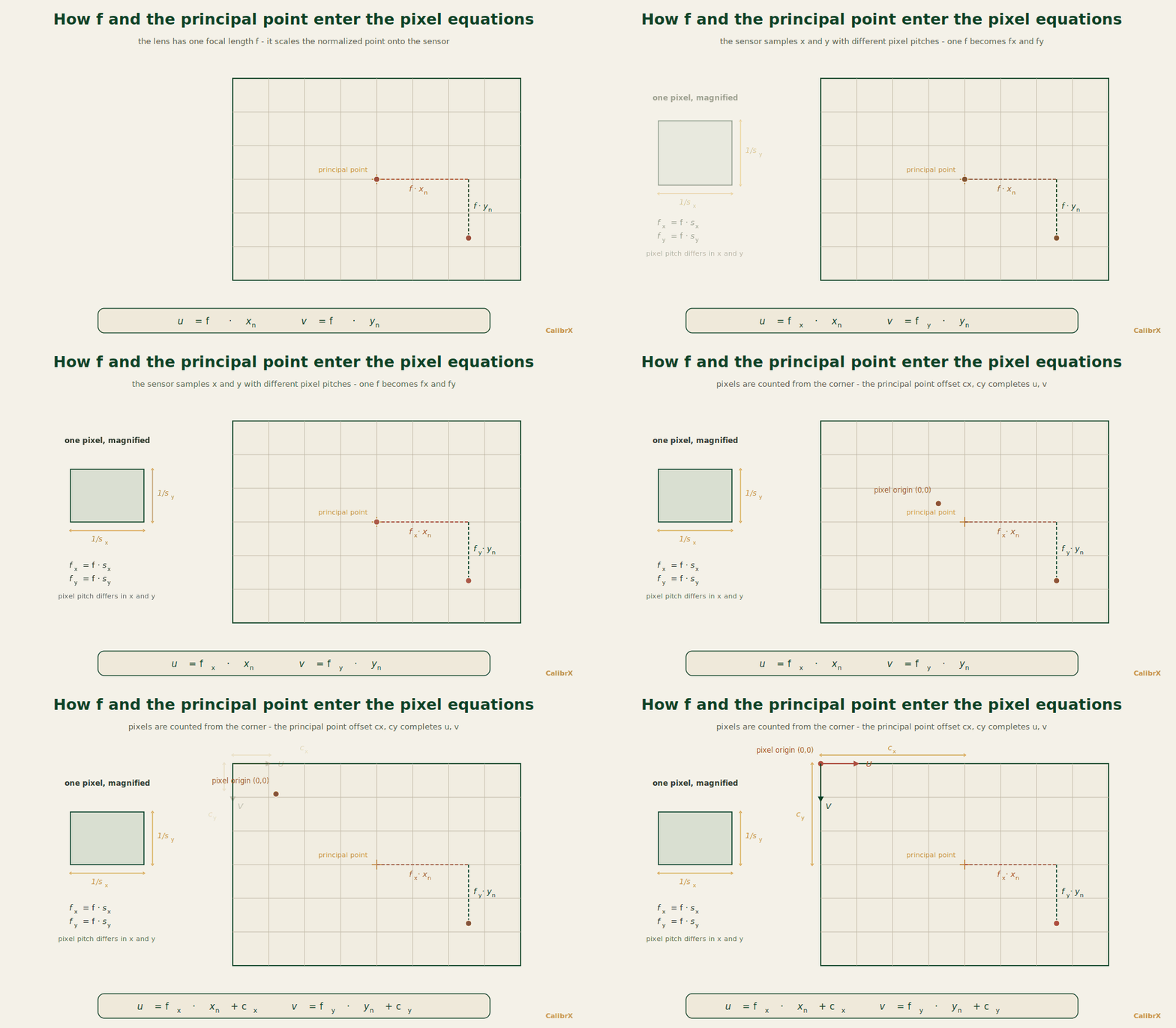
Chaining all four steps in homogeneous coordinates gives the full ideal pinhole model in a single line: Note the on the left-hand side: that is the perspective divide from step three, hiding in plain sight. One computes the right-hand side and divides by the third component to obtain the pixel . Counting parameters, the model has 11 degrees of freedom — 5 intrinsic () and 6 extrinsic (3 for , 3 for ).
One deliberate omission: real lenses are not ideal pinholes. Between the perspective divide and the intrinsic matrix, the lens bends the normalized coordinates — radial and tangential distortion — and this bending is nonlinear, so it cannot be absorbed into . We treat it in detail in a later section; for the structure of the mapping, the ideal model above is the skeleton everything else hangs on.
Calibration, then, is the estimation problem this chain defines: recover the intrinsic parameters (and distortion coefficients) that are fixed properties of the camera, and — usually as a byproduct — the per-image extrinsics describing where the camera stood for each frame used in the solve. Once the intrinsics are known, the chain can be run in both directions: undistorting images, projecting world points to pixels, triangulating from stereo pairs, and estimating pose from known features. None of those are possible without first answering: what camera am I dealing with?
![The same 3D point P shown in both the world frame and the camera frame, related by the extrinsic transform [R | t], with the ray from P through the optical centre C crossing the image plane at pixel (u, v)](/blog/science-camera-projection-overview.svg)
The pinhole model
The simplest geometric model of a camera is the pinhole: imagine all light passing through a single infinitesimal aperture at the camera centre , then landing on a planar sensor at distance (the focal length) behind it. Using the virtual-image convention, where the sensor sits between and the world, similar triangles give the projection equations
Written in homogeneous coordinates and rolled together with the extrinsics, this gives the standard pinhole equation where is a homogeneous world point and is its homogeneous pixel coordinate. The intrinsic matrix does the work of converting metric image-plane coordinates into pixel coordinates.
In pixels rather than metres, the focal length splits into and (the metric focal length divided by the horizontal and vertical pixel pitch). The principal point is where the optical axis pierces the sensor — close to but rarely exactly at the image centre. Together, are the four intrinsic parameters of an ideal pinhole camera.
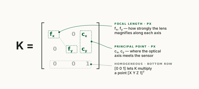
Why distortion exists
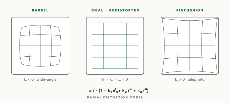
A real lens is not an infinitesimal pinhole. It is a stack of curved glass elements designed to gather more light and project a sharp image. That design introduces deviations from the pure pinhole projection — most prominently, radial distortion, where points appear shifted along the radial direction from the optical centre. Wide-angle and fisheye lenses bow lines outward (barrel distortion), while telephoto lenses can bow them inward (pincushion).
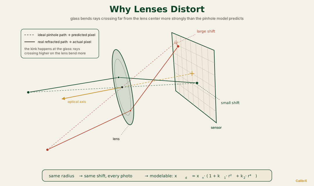
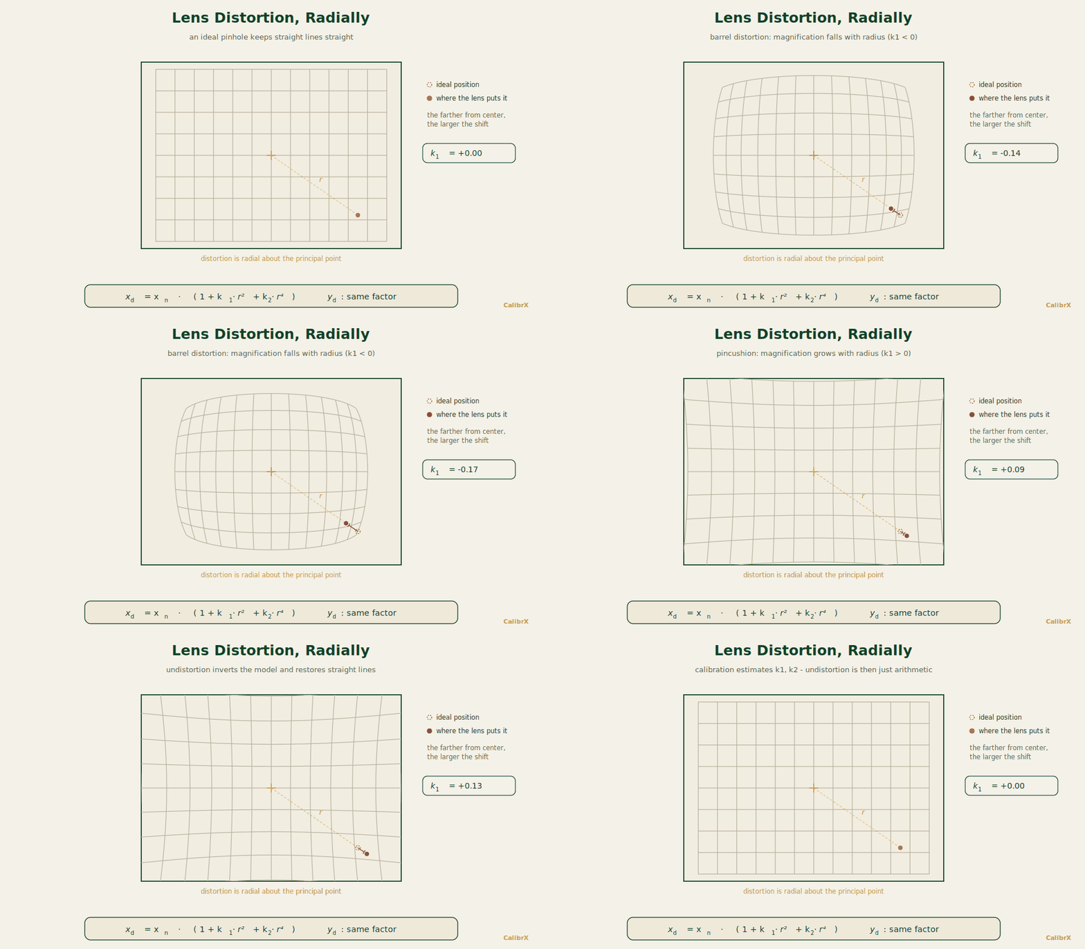
OpenCV models radial distortion with a polynomial in the radial distance from the principal point: Most reasonable lenses are captured by and ; is added for wide-angle. The rational model extends this with in a denominator polynomial for cameras with stronger distortion. Fisheye lenses use a different model entirely — the equidistant projection — because the polynomial approach breaks down near 180°.
There is also tangential distortion, parameterised by and , which appears when the lens elements are not perfectly parallel to the sensor. It is usually small for modern cameras but matters for high-precision work. The full distortion vector is what calibration estimates alongside .
The calibration problem, stated formally
Calibration is an optimisation. We capture images of a planar target whose 3D coordinates are known by construction (a chessboard, ChArUco board, or circles grid). In each image we detect the projections of those known points. The unknowns are: the intrinsics and distortion (shared across all images), and a per-image rigid pose .
The goal is to find the parameters that make the predicted projections match the observations as closely as possible, in the sense of squared pixel distance. Concretely:
This is a nonlinear least-squares problem because is nonlinear in the unknowns (the distortion polynomial is the obvious source of nonlinearity, but rotation is also). The standard solver is Levenberg–Marquardt, initialised from a closed-form solution that ignores distortion. The closed-form initialisation is Zhang's contribution from his 2000 paper: he showed that the homographies between a planar target and its images give linear constraints on , after which distortion can be added back and the whole thing refined nonlinearly.
Reading reprojection error
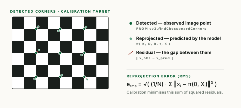
The standard quality metric is the root mean square reprojection error: where is the total number of point observations and is the full parameter vector. This is the same quantity the optimiser was minimising, evaluated at the converged solution. It has units of pixels.
What counts as "low"? It depends on the application. For typical machine-vision lenses on a moderate-resolution sensor, an RMS below is excellent, – is good, and above usually means weak frames, wrong board parameters, or a model mismatch (e.g. trying to fit a fisheye lens with a pinhole model). For sub-pixel measurement work in metrology, sub- is the target.
The trap is that one number can hide a lot. A run can show a respectable average while one or two outlier frames carry most of the error, or while the error is concentrated near the edges of the sensor where the distortion model is failing. That is why analytics that show per-image error, sensor coverage, and residual heatmaps are essential — and why CalibrX surfaces all three.
Three camera models, three trade-offs
In practice, "the pinhole model" is one of several models. Choosing the right one matters: a wide-angle lens fit with a strict pinhole will end up with a high RMS and ugly undistortion at the edges, while a normal lens fit as fisheye will produce parameters with strange physical meaning.
The three families most commonly used: the standard pinhole (Brown-Conrady distortion, OpenCV’s calibrateCamera) for moderate lenses up to roughly 90° field of view; the rational pinhole (additional k₄, k₅, k₆ in a denominator polynomial) for wide-angle lenses up to about 120°; and the equidistant fisheye model (Kannala–Brandt or OpenCV’s fisheye namespace) for true fisheye projections approaching 180°. CalibrX surfaces all three so you can solve the same captures against each and compare RMS and undistorted previews directly.
- Pinhole — standard rectilinear lenses, 4 to 8 distortion coefficients.
- Pinhole wide — rational distortion model for wide-angle and action cameras.
- Fisheye — equidistant projection (Kannala–Brandt) for dome and 180° lenses.
What the parameters let you do
Once calibration has converged, K and D are the keys to every geometric operation the camera can support. Undistorting an image becomes a function call that takes pixels in and pixels out with straight lines preserved. Projecting a 3D world point becomes deterministic. Triangulating depth from a stereo pair requires both cameras’ intrinsics and the rectification homography that aligns their epipolar lines.
For applications that consume the calibration — robotics, drones, AR, 3D reconstruction, machine vision — the export needs more than the raw numbers. It needs the model identifier (pinhole, pinhole_wide, fisheye), the image size used during solving, and ideally the RMS and per-image quality metadata. That structured export is what CalibrX writes to JSON or YAML, and what the calibrx Python SDK reads back to drive undistortion locally with the correct model-specific routine.
Further reading
- Zhang, Z. — A Flexible New Technique for Camera Calibration (2000)The paper that made planar-target calibration practical for any flat board. Underpins OpenCV’s calibrateCamera.
- OpenCV — Camera calibration with OpenCVThe official tutorial covering K, D, the calibration pipeline, and undistortion in OpenCV.
- OpenCV calib3d module referenceAPI reference for calibrateCamera, undistort, projectPoints, and the rational distortion model.
- Kannala & Brandt — A Generic Camera Model and Calibration Method (2006)The equidistant fisheye model used by OpenCV’s cv2.fisheye namespace for wide and 180° lenses.
- Hartley & Zisserman — Multiple View Geometry in Computer VisionThe canonical textbook on projective geometry, camera models, calibration, and multi-view reconstruction.
- CalibrX — camera calibration softwareRun the pinhole, wide, and fisheye calibration described here in the browser: upload images, detect patterns, validate accuracy, and export calibration files.